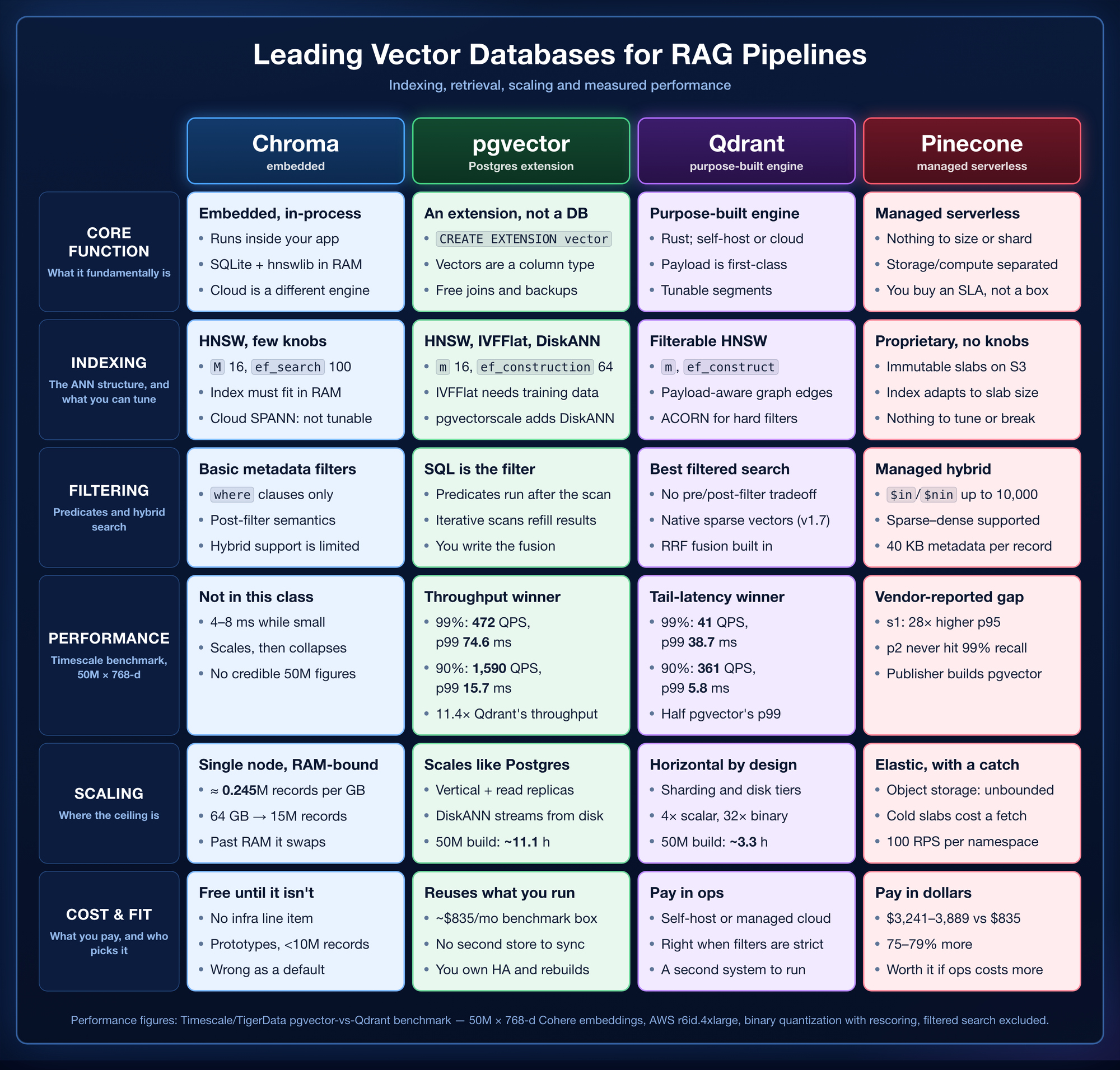
Most teams pick a vector database twice. The first time is on day three of a prototype, when someone types pip install chromadb because it is the shortest path to a working retrieval loop. The second time is eight months later, at 2am, when that same process has a 40 GB resident set and the box has started swapping.
The decision in between never happens. And when it finally does get revisited, it usually gets made on the wrong evidence — a benchmark leaderboard, a conference talk, a table in a blog post that looks a lot like the one above. Leaderboards measure a workload. The question is whether it is your workload.
This post is the long version of that decision. It covers what these four systems actually do differently at the index level, why the published benchmark numbers point in opposite directions depending on who published them, and how to keep the choice reversible so that being wrong costs you a deploy rather than a quarter.
Two operations, and everything else is secondary
Strip away the marketing and a vector database does two things:
- Store a high-dimensional float array with an identifier and some metadata.
- Given a query array, return the k stored arrays closest to it under some distance metric — fast, and usually approximately.
That is it. Everything else — the SDK ergonomics, the LangChain integration, the dashboard, the managed control plane — is packaging around those two operations. Which matters, because packaging is where these four products differ most visibly and least importantly.
The word doing the heavy lifting in operation two is approximately. Exact nearest-neighbour search over a million 768-dimensional vectors means a million dot products per query. That is a linear scan, it is embarrassingly parallel, and on a modern CPU it is also completely impractical past a few hundred thousand vectors if you want single-digit millisecond responses.
So every one of these systems gives up exactness. They build an index that answers “close enough, most of the time,” and the entire engineering conversation is about the shape of that compromise: how much recall you sacrifice, how much memory you spend, how long the index takes to build, and how gracefully the whole thing degrades when you add a WHERE clause.
The index is the product
Four index families show up across these four databases. Understanding them is most of the work, because the vendor differences downstream are largely consequences of which family they bet on.
HNSW — the default everywhere
Hierarchical Navigable Small World graphs are what Chroma uses, what Qdrant uses, and what pgvector uses by default. The structure is a stack of proximity graphs. The bottom layer contains every vector, each connected to its m nearest neighbours. Each layer above is a sparser sample of the one below, with longer-range edges.
Search starts at an entry point in the top, sparse layer and greedily walks toward the query — always stepping to the neighbour that reduces distance most. When it can no longer improve, it drops a layer and repeats with a denser graph and shorter hops. The top layers do coarse navigation across the space; the bottom layer does fine-grained refinement. It is a skip list for metric spaces.
Three parameters control it, and they are the same three everywhere:
m(Chroma calls itmax_neighbors) — edges per node. More edges mean better connectivity and higher recall, at the cost of memory and build time. pgvector and Chroma default to 16; Qdrant’s default is 16 and the Timescale benchmark ran it at 32.ef_construction— how many candidates the builder considers when choosing each node’s neighbours. Higher means a better graph and a slower build. pgvector defaults to 64, Chroma to 100.ef_search(Qdrant:hnsw_ef) — the size of the candidate list at query time. This is the only one you can change after the fact, and it is the recall/latency dial. pgvector defaults to 40, Chroma to 100.
The important structural fact about HNSW: it wants to be in RAM. The access pattern is a pointer chase through a graph, which is close to the worst possible pattern for a block device. This single property explains most of Chroma’s scaling story and a good chunk of pgvector’s.
IVFFlat — the cheap alternative
pgvector’s other built-in index partitions the vector space into lists clusters via k-means, then stores each vector in its nearest cluster’s posting list. A query finds the nearest few cluster centroids and scans only those lists. probes controls how many it scans.
The trade is straightforward: IVFFlat builds much faster and uses much less memory than HNSW, and it returns worse results at equivalent speed. It also needs representative data present at build time in order to train the centroids, which means you cannot create it on an empty table and you should rebuild it after the data distribution shifts substantially. pgvector’s guidance is lists = rows / 1000 below a million rows and sqrt(rows) above it, with probes starting around sqrt(lists).
In practice IVFFlat is the right call when your index does not fit in memory and you cannot use DiskANN, or when build time genuinely dominates. Otherwise HNSW wins.
DiskANN / Vamana — designed for the SSD
This is the interesting one, and it is why the benchmark result later in this post is counterintuitive.
DiskANN — from Microsoft Research, built on a graph called Vamana — starts from a different premise than HNSW. Instead of assuming the index lives in memory, it assumes the index lives on an NVMe SSD and is designed to minimise the number of random reads per query. It is a single flat graph rather than a hierarchy, built with a pruning rule that deliberately keeps some long-range edges so that greedy search converges in few hops. Fewer hops means fewer disk reads.
The pgvectorscale extension brings a streaming variant of this to Postgres, paired with Statistical Binary Quantization — a refinement of ordinary binary quantization that encodes each dimension as one or two bits, chosen using the statistical distribution of that dimension rather than a fixed threshold at zero. The compressed codes stay in memory and drive the graph traversal; full-precision vectors stay on disk and are used to rescore the shortlist at the end.
The result is an index roughly an order of magnitude smaller than HNSW over the same data, that tolerates spilling to disk, and that parallelises well across many concurrent queries. Hold that last clause — it matters in the benchmark section.
SPANN — partition, then graph
Distributed Chroma and Chroma Cloud use SPANN, based on the SPFresh line of work. SPANN splits the difference between IVF and graph methods: a small in-memory index over cluster centroids routes a query to a handful of posting lists, and those posting lists live on disk. The design target is explicitly the case where the full index cannot fit on one machine.
Worth being precise about what this means for the comparison: Chroma Cloud is not the same engine as the Chroma you pip install. They share an API. They do not share an index, a storage layer, or a scaling story. Benchmarks or experience with one tell you very little about the other, and Chroma does not currently expose SPANN’s configuration for tuning.
Chroma: correct for development, and that is the whole point
Chroma in local mode is SQLite for records plus a fork of hnswlib for the index, running inside your Python process. There is no server, no network hop, no connection pool. For a prototype this is close to ideal — the entire retrieval layer is a directory on disk that you can delete and rebuild in seconds.
The limits are documented, specific, and worth memorising before you deploy anything. Chroma’s own guidance gives a linear capacity formula for 1024-dimensional embeddings with a few metadata fields:
| Instance RAM | Practical maximum records |
|---|---|
| 2 GB (documented minimum) | ~250,000 |
| 8 GB | ~1,700,000 |
| 32 GB | ~7,500,000 |
| 64 GB | ~15,000,000 |
The rule of thumb behind it: maximum collection size in millions ≈ 0.245 × RAM in gigabytes, with at least a gigabyte reserved for the system. Query latency in that regime is genuinely good — 4 to 8 ms mean, with 99.9th percentiles between 7 and 33 ms — and it grows roughly linearly with collection size.
What makes it a production hazard is not the ceiling. It is the shape of the failure at the ceiling. HNSW’s memory layout does not page gracefully. When the index no longer fits, the operating system starts swapping a structure whose entire access pattern is random pointer chasing, and latency does not degrade — it collapses. You do not get a warning band where things are slow but serviceable. You get a system that was fine yesterday and is unusable today.
Two smaller operational notes. Queries parallelise up to the vCPU count and then queue linearly, so concurrency past your core count buys nothing. And inserts want batches: anything from 50 to 250 is reasonable, with throughput plateauing around 150 as the CPU saturates.
Use it for prototypes, notebooks, single-developer projects, evaluation harnesses, and anything comfortably under a few million records where you control the growth curve. Do not use it as a production default that you will “migrate later,” because later is defined by an incident.
pgvector: the case for not adding a database
pgvector is an extension, not a database. That sentence is the entire argument for it. CREATE EXTENSION vector gives you a column type, four distance operators, and two index methods. Everything else — transactions, joins, replication, point-in-time recovery, your existing backup rota, your existing monitoring, your existing on-call runbook — you already have.
The storage layout is worth internalising because it drives the capacity math:
| Type | Bytes per value | Max dimensions | Use |
|---|---|---|---|
vector | 4 × dims + 8 | 2,000 | Full float32 precision |
halfvec | 2 × dims + 8 | 4,000 | float16 — half the storage, usually negligible recall loss |
bit | dims / 8 + 8 | 64,000 | Binary quantization, Hamming/Jaccard distance |
sparsevec | 8 × non-zero + 16 | 16,000 non-zero | Sparse/lexical representations |
Ten million 768-dimensional vectors is 30.8 GB as vector, 15.4 GB as halfvec, and 1.04 GB as bit — before the index. That last column is why quantization is not an optimisation you add later; it is a design decision that determines which instance sizes are even on the table.
The distance operators are <-> (L2), <=> (cosine), <#> (negative inner product) and <+> (L1), with <~> and <%> for Hamming and Jaccard on bit vectors. The index only helps when the operator in your ORDER BY matches the operator class the index was built with — a mismatch produces a silent sequential scan, not an error.
Two of those knobs are worth calling out. m and ef_construction are fixed when the index is created and cannot be changed without a full rebuild, so they are a commitment rather than a setting. hnsw.ef_search is a session variable, which makes it the one accuracy dial you can turn per connection — raise it for recall, lower it for latency. Build time is governed by maintenance_work_mem and max_parallel_maintenance_workers; if the graph does not fit in the former, the build gets dramatically slower and the resulting index is worse.
There is one behaviour here that is the single most common way a pgvector deployment is quietly broken. Filters are applied after the index scan, not during it. The HNSW walk returns its LIMIT worth of candidates by pure vector distance; the WHERE clause then discards whichever of them fail the predicate. Ask for ten results with a selective tenant filter and you may get three — not an error, not a warning, just a shorter list and an answer with less context than you designed for.
Iterative index scans, added in pgvector 0.8, are the fix: the scan resumes and fetches more candidates until the limit is satisfied or a tuple budget is exhausted. relaxed_order allows slight reordering for better recall; strict_order preserves exact distance ordering at higher cost. If you filter at all — and everyone with multi-tenancy filters — this is not optional configuration.
The honest weaknesses: index builds are slow and memory-hungry, HNSW build quality depends on the graph fitting in maintenance_work_mem, and pgvectorscale‘s DiskANN build is currently single-threaded. There is no native sparse-vector fusion; you can combine tsvector full-text search with vector search in SQL, but you write the fusion logic yourself. And every vector operation competes for the same buffer cache as your OLTP traffic, which is fine until it isn’t.
Qdrant: what a purpose-built engine actually buys
Qdrant is a search engine written in Rust whose central design decision is that vectors and structured payload are equal citizens. Data lives in segments, each independently indexed and optimised, which is what lets the storage tiering and the horizontal sharding work.
Three things distinguish it in practice.
Filterable HNSW. Covered in detail in the next section, but the short version is that Qdrant builds payload-aware edges into the graph at construction time, so filtered search does not fall back to either of the two bad strategies everyone else uses.
Quantization with rescoring as a first-class path. Scalar quantization maps float32 to int8 for a 4× reduction. Binary quantization takes each dimension to a single bit for up to 32×, and because comparison becomes a XOR and a popcount, it is dramatically faster as well as smaller. The accuracy loss is recovered by oversampling — pulling, say, twice as many candidates using the cheap codes — and then rescoring that shortlist against full-precision vectors held on disk. You pay one sequential read at the end of the query instead of carrying full precision through the whole traversal.
Explicit memory tiering. Indexes can be pinned (always resident), cached (in the disk cache, evictable under pressure), or cold (on disk, loaded on demand). Combined with is_tenant and is_principal payload indexes — which physically colocate a tenant’s data, or order storage by a timestamp field — this gives you real control over what occupies RAM in a multi-tenant system.
One ordering constraint deserves emphasis, because it is expensive to discover late. Qdrant only builds filter-aware graph edges for fields that are indexed at the time the HNSW graph is constructed. Add the payload index after ingesting a hundred million points and you have an index that answers filter predicates but a graph that knows nothing about them — you need a rebuild to get the benefit. This is an easy and expensive mistake.
The cost of Qdrant is simply that it is a second stateful system. Another thing to deploy, monitor, back up, upgrade, and reason about during an incident. If your data already lives in Postgres, you are also now responsible for keeping two stores consistent, which is a distributed systems problem you did not have yesterday.
Pinecone: paying to not think about it
Pinecone serverless is architecturally the most different of the four. Records compact into immutable files called slabs that live in object storage. Writes go to a log with a sequence number and return 200 OK as soon as they are durable; an index builder asynchronously moves data from an in-memory memtable into slabs and merges small slabs into larger ones over time. Reads go through a query router to executors that fetch and cache the relevant slabs locally.
A freshness layer tails the same log so that recent writes are searchable before they have been compacted — and reads check the memtable first, which is what gives you read-your-writes behaviour rather than the eventual consistency you might expect from an object-storage-backed system.
The consequences are worth stating plainly:
- Capacity is effectively unbounded and read/write paths scale independently, because they are genuinely different services.
- Latency is bimodal. A query against cached slabs is fast. A query that touches a cold slab pays an object-storage fetch. For steady traffic against a hot working set this rarely matters; for sparse access across a very large index it absolutely does.
- You cannot tune the index. No
m, noef_search, no quantization choice. This is the product working as intended — it is also the reason a workload with unusual recall requirements can hit a wall you have no lever against.
The documented limits that most often surprise people: 40 KB of filterable metadata per record, top_k capped at 10,000 with a 4 MB result ceiling, upserts capped at 2 MB or 1,000 records per request, $in/$nin arrays capped at 10,000 values, and — the one that catches people building high-throughput pipelines — a default of 100 requests per second per namespace for queries, upserts and deletes alike. That is adjustable on request, but it needs to be discovered before launch rather than during it.
The filtering problem, which is where most RAG systems actually die
Pure vector search is a solved problem. Vector search with a predicate is not, and almost every real system has predicates: tenant isolation, document ACLs, date ranges, language, source, status.
There are two obvious strategies and both are bad.
Post-filtering runs the ANN search first and applies the predicate to the results. It is trivial to implement and it breaks precisely when the filter is selective. If one percent of your corpus belongs to this tenant, retrieving 10 by vector similarity and then filtering leaves you with roughly nothing. You compensate by over-fetching — retrieve 1,000, filter, keep 10 — which works until the selectivity gets worse, at which point you are over-fetching 100,000 and have reinvented the linear scan with extra steps.
Pre-filtering applies the predicate first and searches only the surviving subset. This guarantees correct results, and it destroys the index. HNSW’s graph connectivity assumes all its nodes are present; remove most of them and the greedy walk strands itself in disconnected components. In practice pre-filtering degenerates to a brute-force scan over the filtered set, which is fine for a thousand rows and catastrophic for ten million.
This is the actual differentiator between these four systems.
- Chroma offers metadata
whereclauses with effectively post-filter semantics. - pgvector post-filters by construction — the predicate is a SQL
WHEREevaluated on rows the index scan already returned — with iterative scans as the mitigation. - Pinecone handles filtering inside the managed index, with the metadata size and
$incardinality limits noted above. - Qdrant attacks the problem structurally. When payload indexes exist at build time, it adds extra edges to the HNSW graph connecting points that share indexed payload values. The graph stays navigable under a filter because the filter-satisfying subgraph was explicitly given its own connectivity. For hard multi-predicate cases where those edges are still insufficient, ACORN (v1.16+) explores neighbours-of-neighbours when direct neighbours are filtered out, trading throughput for accuracy.
This is an active research area rather than a settled one. The literature includes ACORN, Filtered-DiskANN (in FilteredVamana and StitchedVamana variants), UNG, Curator and SIEVE, and recent benchmark work is fairly blunt that no method dominates: specialised approaches often beat ACORN, while several methods that look excellent at medium scale fail outright on large transformer-embedding datasets. The practical takeaway is not “Qdrant wins filtered search” — it is that if your workload is filter-heavy, you must benchmark filtered queries specifically, because unfiltered numbers will not predict them.
Hybrid search: the other half of retrieval quality
Dense vectors are bad at exact matches. Part numbers, error codes, proper nouns, rare acronyms — the embedding puts them in a neighbourhood of semantically similar things, which is exactly wrong when the user typed a literal identifier. Sparse lexical retrieval (BM25 and its learned successors like SPLADE) is good at precisely that and bad at paraphrase. Combining them, usually with Reciprocal Rank Fusion, reliably beats either alone.
Support here is genuinely uneven, and it is the dimension the comparison table above compresses most:
- Qdrant — native sparse vectors since v1.7, dense and sparse in one collection, RRF and weighted linear fusion in the Query API. The cleanest of the four.
- Pinecone — sparse-dense hybrid supported within the managed index.
- pgvector — no sparse fusion primitive. You can absolutely run
tsvectorfull-text alongside vector search and fuse in SQL or in application code, and plenty of production systems do, but you are writing and maintaining that logic. - Chroma — limited.
RRF at k=60 is the sensible default. It ranks rather than scores, so it needs no normalisation between two systems whose score distributions have nothing in common.
The benchmark, and why its result is counterintuitive
The most-cited head-to-head here is Timescale’s, and it is worth walking through carefully because the shape of the result is more instructive than the winner.
Setup: 50 million Cohere embeddings at 768 dimensions, 1,000 test queries, AWS r6id.4xlarge (16 vCPU, 128 GB RAM, 950 GB NVMe), about $835/month. pgvectorscale ran StreamingDiskANN with SBQ and a rescore depth of 400. Qdrant ran HNSW at m=32, ef_construct=64, hnsw_ef=768, with binary quantization and rescoring enabled.
| At 99% recall | pgvectorscale | Qdrant |
|---|---|---|
| p50 latency | 31.07 ms | 30.75 ms |
| p95 latency | 60.42 ms | 36.73 ms |
| p99 latency | 74.60 ms | 38.71 ms |
| Throughput | 471.57 QPS | 41.47 QPS |
| Index build time | ~11.1 hours | ~3.3 hours |
| At 90% recall | pgvectorscale | Qdrant |
|---|---|---|
| p50 latency | 9.54 ms | 4.74 ms |
| p95 latency | 13.30 ms | 5.50 ms |
| p99 latency | 15.73 ms | 5.79 ms |
| Throughput | 1,589.79 QPS | 360.81 QPS |
Read those two tables again. Qdrant wins every latency percentile. pgvectorscale wins throughput by 11.4×. Both are true simultaneously, and if your instinct is that one of them must be a measurement error, that instinct is what this section exists to correct.
Latency and throughput answer different questions. Latency is how long one query takes when the system is not fighting itself. Throughput is how many queries the system completes per second when it is fully loaded — which is a question about parallel efficiency, not about single-query speed.
The architectures explain the split. Qdrant at 99% recall needed hnsw_ef=768 — an enormous candidate list. Each query does a large amount of tightly-coupled graph traversal work, and it does it very consistently, which is exactly why the tail is tight: p50 30.75 ms to p99 38.71 ms is a spread of eight milliseconds. Predictability is the signature of a well-fed in-memory graph walk.
StreamingDiskANN is doing something structurally different. It traverses a compressed in-memory graph, then rescores 400 candidates against full-precision vectors on NVMe. Any individual query has more variance — hence p99 nearly two and a half times p50 — but Postgres runs each connection in its own process, the SSD handles deep parallel queues well, and sixteen cores stay saturated. The design optimises aggregate work done, not the worst case for any one request.
So which number matters is a product question, not an engineering one. A user-facing chatbot lives and dies by p99, because the tail is what people experience as “it’s slow.” A nightly batch enrichment job over ten million documents cares only about total throughput and would happily accept a 75 ms p99. Picking the database that wins the metric you do not care about is the most common way this decision goes wrong.
Reading benchmarks honestly
Four caveats, three of which the authors state themselves.
The publisher matters. That benchmark is published by Timescale, who build pgvectorscale. Qdrant publishes its own benchmark suite — against Elasticsearch, Milvus, Redis and Weaviate on dbpedia-openai-1M, deep-image-96, gist-960 and glove-100 — and concludes that Qdrant achieves the highest RPS and lowest latencies in almost every scenario. Notably, pgvector is not in that comparison set. Neither party is lying. Both are reporting real measurements from configurations they understand well and their competitor’s less well.
Tuning effort is asymmetric and admitted. The Timescale authors state directly that it was time-prohibitive to test all Qdrant configurations and that they may have missed a better set of values. That is an honest disclosure, and it is also a structural feature of every vendor benchmark ever published.
Filtered search was excluded. The benchmark tested unfiltered ANN queries only. That omission removes the exact workload where Qdrant’s filterable HNSW is designed to be differentiating — so on filter-heavy traffic, these numbers do not merely under-describe Qdrant, they may invert.
One instance type, one dataset, one dimensionality. 50M × 768-d on a machine with 128 GB of RAM and fast local NVMe. Change any of those and the ranking can move: less RAM favours the disk-resident design, more RAM favours the in-memory graph, a different dimensionality changes the quantization arithmetic entirely.
The Pinecone comparison from the same source follows the same pattern and deserves the same scepticism: pgvectorscale reported at 28× lower p95 and 16× higher throughput than Pinecone’s s1 at 99% recall, and 1.4×/1.5× better than p2 at 90% — with the note that p2 could not reach 99% recall at all. On cost, $835/month self-hosted against $3,241 for s1 and $3,889 for p2. That cost gap is real and large. It also excludes the engineer who keeps the Postgres box alive, which for many teams is the more expensive line item.
If you take one operational habit from this post: run VectorDBBench against your own embeddings, your own filter distribution and your own hardware. It supports 30+ engines, it has explicit filtered-search and streaming cases, and it reports QPS, p50/p95/p99, recall, build time and a cost-normalised QP$ metric. A day of that is worth more than every leaderboard in this post.
Where each one actually breaks
Failure modes are more useful than feature matrices, because you will meet these.
| System | What breaks | What it feels like |
|---|---|---|
| Chroma | Index exceeds RAM | No degradation band — fine yesterday, swapping and unusable today |
| pgvector | Selective filters without iterative scans | Silently short result sets; RAG answers get vaguer with no error anywhere |
| pgvector | Index build at scale | Eleven hours, single-threaded, competing with production for buffer cache |
| Qdrant | Payload index created after ingest | Filters work, filtered search is slow, and fixing it means rebuilding the graph |
| Qdrant | Second stateful system | Dual-write consistency, a second backup story, a second thing to page you |
| Pinecone | 100 RPS per namespace default | Load test hits a wall that has nothing to do with the index |
| Pinecone | Cold slabs, no tuning knobs | Tail latency you cannot engineer around, only escalate about |
Three mistakes that are not about the database at all
The index was never built. Vector search works correctly with no index — it just does a sequential scan. On 50,000 rows in staging this is imperceptible. On 5 million in production it is a timeout. Nothing errors, because nothing is wrong; the query planner made a reasonable choice about a table it had no index for. Assert the index exists in a startup check.
Dimension mismatch after a model change. Swapping embedding models mid-project, or letting a provider default drift, produces vectors of a different width or — worse — the same width from a different latent space. Same-width mismatches do not error. They return confident, plausible, wrong neighbours. Pin the model and the dimension count in code, store both in collection metadata, and refuse to start when they disagree.
Estimating collection size from document count. Teams size infrastructure for “we have 100,000 documents” and forget that chunking multiplies. At 800-token chunks with overlap, a corpus of 100,000 modest documents is comfortably 2–3 million vectors. That is the difference between a laptop and a 32 GB instance, and it is usually discovered after the instance has been provisioned.
The decision, in five questions
Answer these in order and stop at the first one that gives you a clear answer.
- Is this going to production, or is it an experiment? If it is an experiment, use Chroma and stop reading. The time you save is real and the migration cost is low precisely because you have not built anything on it yet.
- Is your operational data already in Postgres? If yes, the default is pgvector, and the burden of proof is on adding a second system. Joining embeddings to the rows they came from — with real transactions and one backup — eliminates an entire class of consistency bug that people routinely underestimate.
- Are your queries filter-heavy or hybrid? Strict multi-tenancy, ACLs, date windows, or a genuine need to fuse BM25 with dense retrieval push hard toward Qdrant. This is the dimension where architecture, not tuning, decides the outcome.
- Is p99 latency a product requirement or a vanity metric? If a user is waiting on the response, the tail is the product, and Qdrant’s consistency has real value. If it is a batch pipeline, throughput wins and pgvectorscale’s numbers are compelling.
- What does an engineer-hour cost you relative to an instance-hour? Pinecone is roughly four times the infrastructure cost in the comparison above. For a team of three shipping a product, “nobody gets paged about the vector database” can be worth considerably more than $2,400 a month. For a team of thirty with a platform group, it usually is not.
The uncomfortable truth underneath all five is that at one million vectors, on modern hardware, all four of these are fast enough. The differences that show up in benchmarks at fifty million are mostly invisible at one, and most RAG systems never reach ten. Which means the decision is usually not about performance at all — it is about operational fit, filter semantics, and who carries the pager.
Keep the choice reversible
Given all of the above, the highest-leverage thing you can do is make the decision cheap to revisit. Depend on a retrieval interface, not a client library, and the vector store becomes an environment variable.
Concretely: put a single factory function behind every call site. It reads one variable — call it VECTOR_STORE — dispatches to a small builder per backend, and returns whatever retriever abstraction your framework provides. Nothing downstream imports a database client; the agent, the chain and the evaluation harness all see the same interface regardless of what is behind it. The embedding model and its dimension count belong in that same function, pinned explicitly, so a backend swap can never quietly become a model swap.
This is not an abstraction for its own sake. It is what lets you develop against Chroma locally with no infrastructure, run integration tests against pgvector in CI, and deploy to Qdrant in production — with one variable and no changes to the agent or the chain that consumes the retriever. It also makes an honest comparison tractable: point the same evaluation set at each backend in turn and measure your own recall on your own filters, which is the only benchmark that was ever going to answer the question.
Two constraints keep it useful. The k and the embedding model must be identical across backends or the comparison is meaningless. And the interface must stay narrow — the moment you leak QdrantVectorStore-specific parameters into a call site, the factory has stopped buying you anything.
Closing thought
The comparison table at the top of this post is useful and slightly dishonest, in the way all such tables are. It presents six dimensions as independent when they are deeply coupled: the index choice determines the memory profile, the memory profile determines the scaling ceiling, the filtering architecture determines whether the latency numbers mean anything for your traffic, and the operational burden determines whether any of it survives contact with a small team.
The four systems are not really competing for the same job. Chroma is a development tool that can serve small production loads. pgvector is a way to avoid adding a database. Qdrant is a search engine for people whose queries have predicates. Pinecone is a way to convert an operational problem into an invoice.
Pick the one whose failure mode you can live with, keep the interface narrow enough to change your mind, and benchmark your own filters before you trust anyone’s numbers — including these.
Sources and further reading. Benchmark figures throughout are from Timescale/TigerData’s pgvector vs. Qdrant benchmark and their pgvector vs. Pinecone comparison. Architecture and limits are from the pgvector repository, Qdrant’s indexing documentation and benchmark suite, Chroma’s single-node performance guide and collection configuration docs, and Pinecone’s serverless architecture and database limits references. For running your own numbers, VectorDBBench. The framing of this post owes a debt to StackOps AI’s Choosing the Best Vector Database For Your RAG Pipeline, which covers the same four systems and the same Timescale study.
Leave a Reply